Distributed Tracing with Jaeger and the ELK Stack

Over the past few years, and coupled with the growing adoption of microservices, distributed tracing has emerged as one of the most commonly used monitoring and troubleshooting methodologies. 

New tracing tools and frameworks are increasingly being introduced, driving adoption even further. One of these tools is Jaeger, a popular open source tracing tool. This article explores the integration of Jaeger with the ELK Stack for analysis and visualization of traces.

What is Jaeger?

Jaeger was developed by Uber and open sourced in 2016. Inspired by other existing tracing tools, Zipkin and Dapper, Jaeger is quickly becoming one of the most popular open source distributed tracing tools, enabling users to perform root cause analysis, performance optimization and distributed transaction monitoring.  

Jaeger features OpenTracing-based instrumentation for Go, Java, Node, Python and C++ apps, uses consistent upfront sampling with individual per service/endpoint probabilities, and supports multiple storage backends — Cassandra, Elasticsearch, Kafka and memory.

From an architectural perspective, Jaeger is comprised of multiple components, three of which provide the core backend functionality: Jaeger Clients implement OpenTracing API in applications, creating spans when receiving new requests. Jaeger Agents are responsible for listening for spans and sending them to the Collector.  The collector, in turn, receives the traces from the agents and runs them through a processing pipeline which ends with storing them in backend storage. 

Jaeger and ELK

The default storage is Cassandra but Jaeger can also store traces in Elasticsearch. This capability means users can analyze traces using the full power of the ELK Stack (Elasticsearch, Logstash and Kibana). Why does this matter?

Sure, Jaeger ships with a nifty GUI that allows users to dive into the traces and spans. Using the ELK Stack, though, offers users additional querying and visualization capabilities. Depending on your ELK architecture, you will also be able to store trace data for extended retention periods. If you’re already using the ELK Stack for centralized logging and monitoring, why not add traces into the mix?

Let’s take a closer look at how to set up the integration between Jaeger and the ELK Stack and some examples of what can be done with it. 

Step 1: Setting Up Elasticsearch and Kibana

Our first step is to set up a local ELK (without Logstash) with Docker. Jaeger currently only supports versions 5.x and 6.x, so I will use the following commands to run Elasticsearch and Kibana.

Elasticsearch 6.8.0:

docker run --rm -it --name=elasticsearch -e "ES_JAVA_OPTS=-Xms2g -Xmx2g"
-p 9200:9200 -p 9300:9300 -e "discovery.type=single-node" -e
"xpack.security.enabled=false"
docker.elastic.co/elasticsearch/elasticsearch:6.8.0

Kibana 6.8.0:

docker run --rm -it --link=elasticsearch --name=kibana -p 5601:5601
docker.elastic.co/kibana/kibana:6.8.0

Step 2: Setting Up Jaeger

Next, we will deploy Jaeger.

Designed for tracing distributed architectures, Jaeger itself can be deployed as a distributed system. However, the easiest way to get started is to deploy Jaeger as an all-in-one binary that runs all the backend components in one single process.

To do this, you can either run the jaeger all-in-one binary, available for download here, or use Docker. We will opt for the latter option.

Before you copy the command below, a few words explaining some of the flags I’m using:

• –link=elasticsearch – link to the Elasticsearch container.
• SPAN_STORAGE_TYPE=elasticsearch – defining the Elasticsearch storage type for storing the Jaeger traces.
• -e ES_TAGS_AS_FIELDS_ALL=true – enables correct mapping in Elasticsearch of tags in the Jaeger traces.

docker run --rm -it --link=elasticsearch --name=jaeger -e
SPAN_STORAGE_TYPE=elasticsearch -e
ES_SERVER_URLS=http://elasticsearch:9200 -e ES_TAGS_AS_FIELDS_ALL=true
-p 16686:16686 jaegertracing/all-in-one:1.12

You can now browse to the Jager UI with: http://localhost:16686

Step 3: Simulating trace data

Great, we’ve got Jaeger running. It’s now time to create some traces to verify they are being stored on our Elasticsearch instance. 

To do this, I’m going to deploy HOT R.O.D  – an example application provided as part of the project that consists of a few microservices and is perfect for easily demonstrating Jaeger’s capabilities.

Again, using Docker:

docker run --rm --link jaeger --env
JAEGER_AGENT_HOST=jaeger --env JAEGER_AGENT_PORT=6831 -p8080-8083:8080-8083
jaegertracing/example-hotrod:latest all

Open your browser at: http://localhost:8080:

Start calling the different services by playing around with the buttons in the app. Each button represents a customer and by clicking the buttons, we’re ordering a car to the customer’s location. Once a request for a car is sent to the backend, it responds with details on the car’s license plate and the car’s ETA:

Within seconds, traces will be created and indexed in Elasticsearch. 

To verify, cURL Elasticsearch:

curl -X GET "localhost:9200/_cat/indices?v"

health status index                     uuid                   pri rep docs.count docs.deleted store.size pri.store.size
green  open   .kibana_1                 LffR3embTkyjs-TdCMQYYQ   1   0          4            0     14.4kb         14.4kb
yellow open   jaeger-span-2019-06-18    Vuujr66CTg6AdPgPkX7xUw   5   1          1            0     11.4kb         11.4kb
green  open   .kibana_task_manager      btmJCT9MQ9ydviiMWgDxCQ   1   0          2            0     12.5kb         12.5kb
yellow open   jaeger-service-2019-06-18 T_lS1JQWT4aozUHxVmY9Tw   5   1          1            0      4.5kb          4.5kb

Step 4: Hooking up Jaeger with ELK

The final step we need to take before we can start analyzing the traces is define the new index pattern in Kibana.

To do this, open the Management → Kibana → Index Patterns page. Kibana will display any Elasticsearch index it identifies, including the new Jaeger index.  

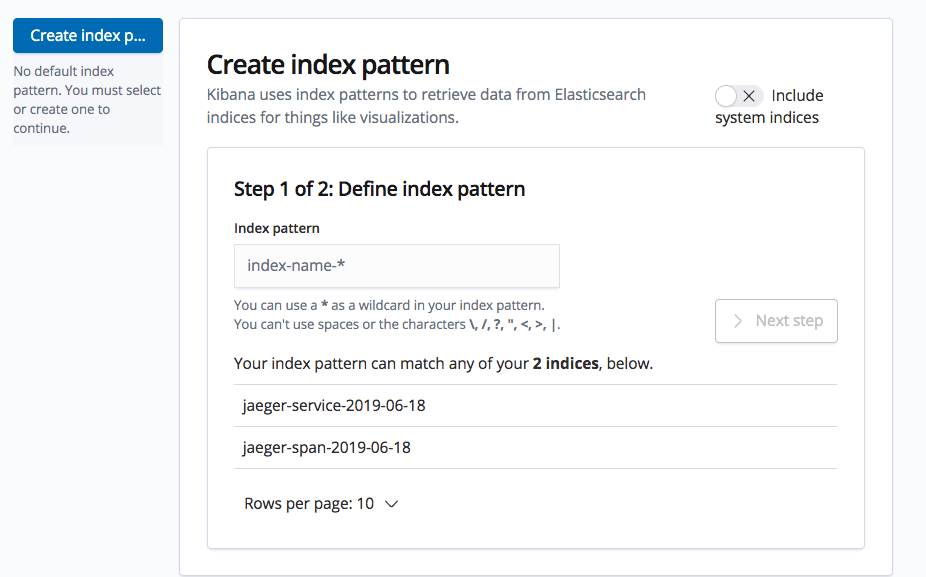
Enter ‘jaeger-span-*’ as your index pattern, and in the next step select the ‘statTimeMillis’ field as the time field.

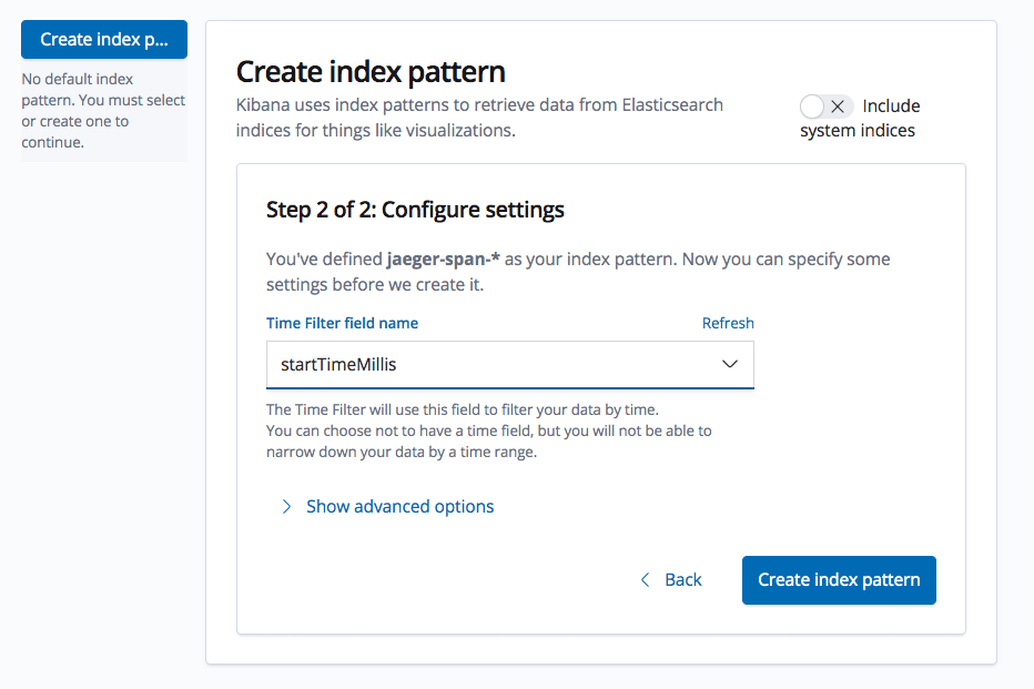
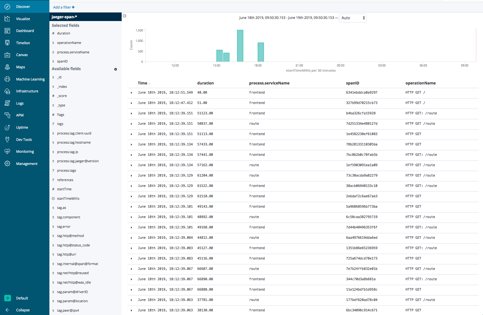
Hit the Create index pattern button and then open the Discover page — you’ll see all your Jaeger trace data as indexed and mapped in Elasticsearch:

Step 5: Analyzing traces in Kibana

You can now start to use Kibana queries and visualizations to analyze the trace data. Kibana supports a wide variety of search options and an even bigger amount of visualization types to select from. Let’s take a look at some examples.

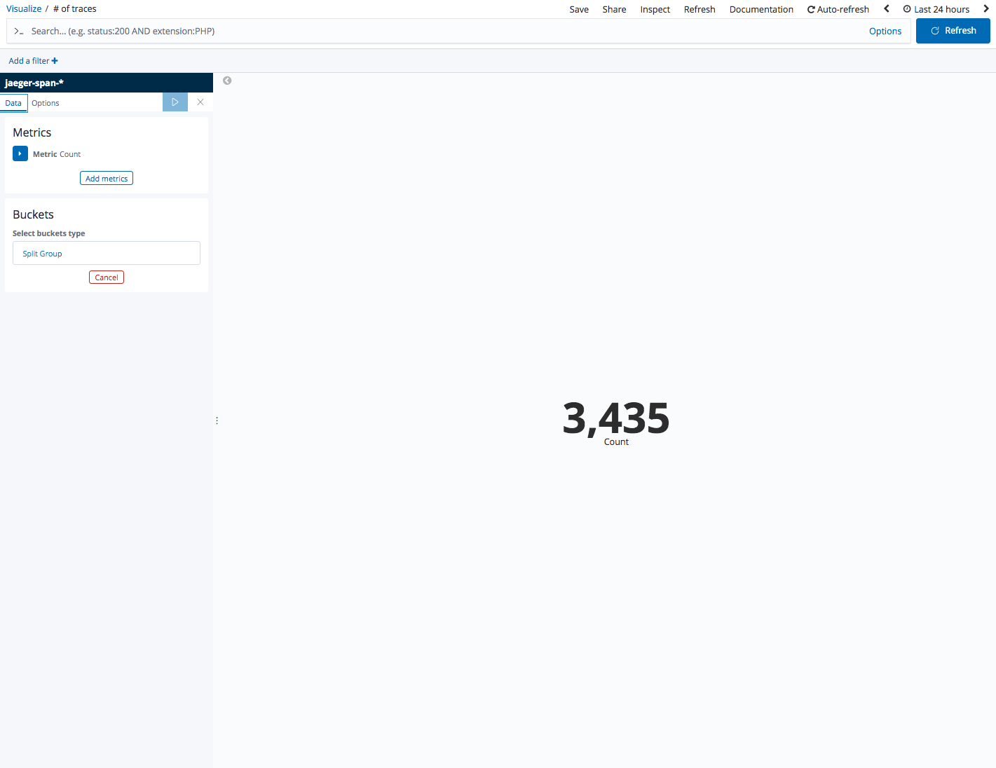
No. of traces

Let’s start with the basics. Metric visualizations are great for displaying a single metric. In the examples below we’re showing the overall number of traces being sampled:

Traces per service

Using a bar chart visualization, we can view a breakdown of the traces per microservice. To build this visualization, use a count aggregation as the Y axis, and a terms aggregation of the process.serviceName field as the X axis.

Avg. transaction duration

Line charts are useful for identifying trends over time. In the example below, we’re using a line chart to monitor the average duration of requests per service. To build this visualization, use an average aggregation of the duration field as the Y axis, together with a time histogram and a split series of the process.serviceName field as the Y axis:

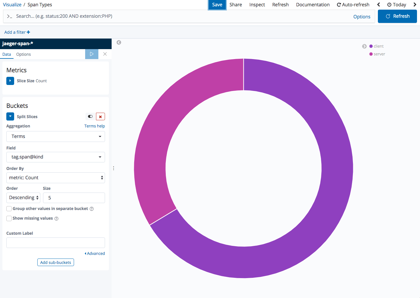
Span types

Pie charts are super simple visualizations that can help view a breakdown of a specific field. In the example below, we’re using a pie chart to visualize the breakdown between client and server requests using a terms aggregation of the tag.span@kind field:

Trace list

Using a saved search visualization, you can insert a list of the actual traces as a visualization in a dashboard. To do this, first save the search in the Discover page. In the example below, I’ve added the duration, process.serviceName, spanID and operationName fields to the main view but you can, of course, add the fields you want to be displayed:

Then, when adding visualizations to your dashboard simply select to add a visualization from a saved search and select the search you saved above.

Adding this visualization, together with all the other visualizations, in one dashboard gives you a nice overview of all the tracing activity Jaeger has recorded and stored in Elasticsearch:

Endnotes

The Jaeger UI does a great job at mapping the request flow, displaying the different spans comprising traces and allowing you to drill down into them. You can even compare different traces to one another. 

Kibana provides users with additional querying and visualization capabilities which give you a more comprehensive view. Again, when combined with logs and metrics — using the ELK Stack with Jaeger is a powerful combination. 

Stay tuned for our future integration with Jaeger, which will enable you to easily analyze traces along with logs and metrics in one unified platform!