A Basic Guide To Elasticsearch Aggregations
August 29, 2019

Elasticsearch Aggregations provide you with the ability to group and perform calculations and statistics (such as sums and averages) on your data by using a simple search query. An aggregation can be viewed as a working unit that builds analytical information across a set of documents. Using aggregations, you can extract the data you want by running the GET method in Kibana UI’s Dev Tools. You can also use CURL or APIs in your code. These will query Elasticsearch and return the aggregated result.More on the subject:
Here are two examples of how you might use aggregations:
- You’re running an online clothing business and want to know the average total price of all the products in your catalog. The Average Aggregation will calculate this number for you.
- You want to check how many products you have within the “up to $100” price range and the “$100 to $200” price range. In this case, you can use the Range Aggregation.
This article will describe the different types of aggregations and how to run them. It will also provide a few practical examples of aggregations, illustrating how useful they can be.
Elasticsearch aggregations can be used on your own self-managed ELK Stack or managed services like Logz.io, which provides OpenSearch and OpenSearch Dashboards (the new, forked versions of Elasticsearch and Kibana, respectively, maintained by AWS) on a fully managed SaaS platform – offloading tasks like cluster management, parsing, upgrading, and other logging infrastructure maintenance requirements.
Getting Started
In order to start using aggregations, you should have a working setup of ELK. If you don’t, step-by-step ELK installation instructions can be found at this link.
You will also need some data/schema in your Elasticsearch index. You can use any data, including data uploaded from the log file using Kibana UI. In this article, we are using sample eCommerce order data and sample web logs provided by Kibana.
To get this sample data, visit your Kibana homepage and click on “Load a data set and a Kibana dashboard.” There, you will see the sample data provided for eCommerce orders and web logs. This process is shown in Screenshots A and B below.


The Aggregation Syntax
It is important to be familiar with the basic building blocks used to define an aggregation. The following syntax will help you to understand how it works:
-----
"aggs”: {
    “name_of_aggregation”: {
      “type_of_aggregation”: {
        “field”: “document_field_name”
}
-----
aggs—This keyword shows that you are using an aggregation.
name_of_aggregation—This is the name of aggregation which the user defines.
type_of_aggregation—This is the type of aggregation being used.
field—This is the field keyword.
document_field_name—This is the column name of the document being targeted.
A Quick Example
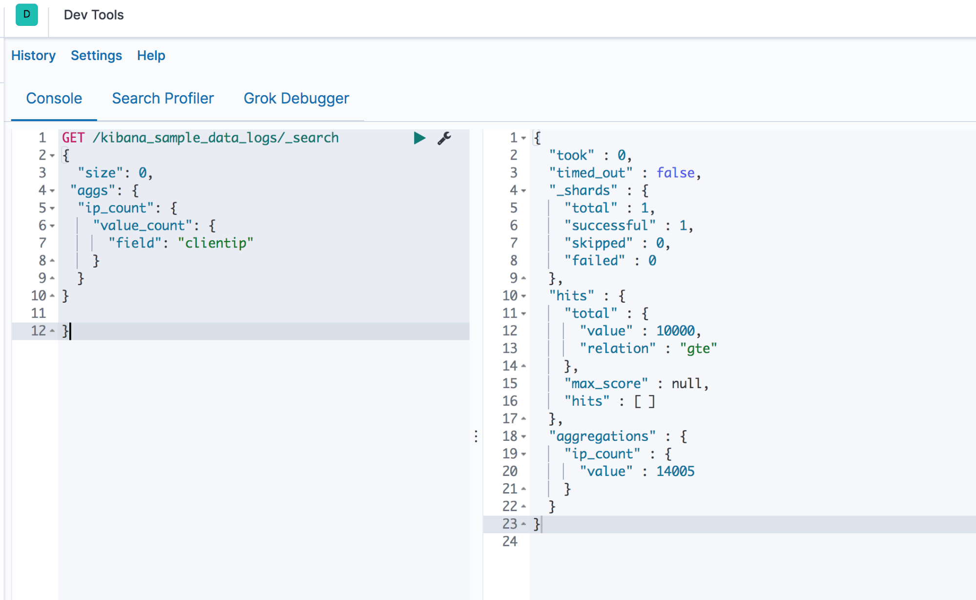
The following example shows the total counts of the “clientip” address in the index “kibana_sample_data_logs.”
The code written below is executed in the Dev Tools of Kibana. The resulting output is shown in Screenshot C.
GET /kibana_sample_data_logs/_search
{ "size": 0,
 "aggs": {
  "ip_count": {
    "value_count": {
      "field": "clientip"
                    }
               }
          }
}
Output
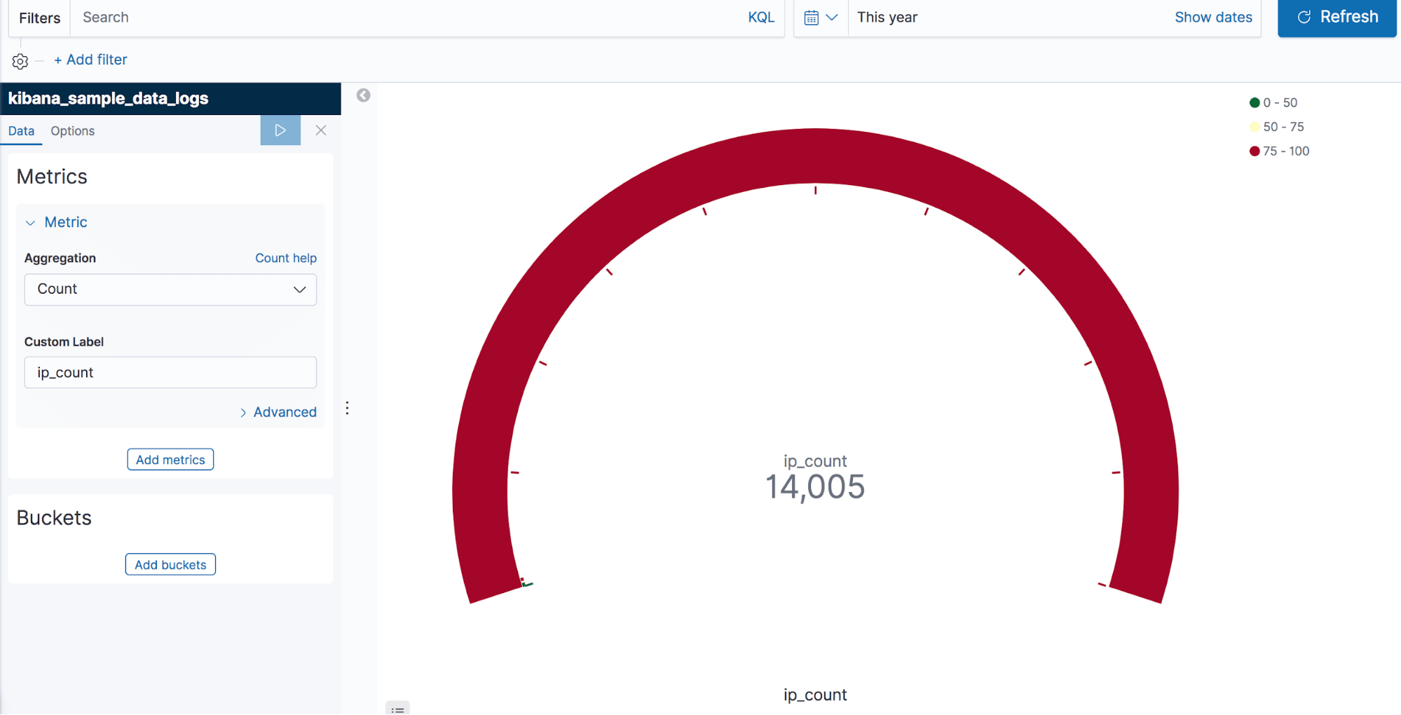
You can also use the Kibana UI to get the same results as shown in Screenshot C. Here, we created a gauge visualization by clicking on the “Visualize” tab of Kibana with the index “kibana_sample_data_logs.” Then, we simply selected the count aggregation from the left-hand pane. Finally, we clicked on the “execute” button.
In Screenshot D, you can see the resulting ip_count value in the gauge visualization.
Key Aggregation Types
Aggregations can be divided into four groups: bucket aggregations, metric aggregations, matrix aggregations, and pipeline aggregations.
- Bucket aggregations—Bucket aggregations are a method of grouping documents. They can be used for grouping or creating data buckets. Buckets can be made on the basis of an existing field, customized filters, ranges, etc.
- Metric aggregations—This aggregation helps in calculating matrices from the fields of aggregated document values.
- Pipeline aggregations—As the name suggests, this aggregation takes input from the output results of other aggregations.
- Matrix aggregations (still in the development phase)—These aggregations work on more than one field and provide statistical results based on the documents utilized by the used fields.
All of the above aggregations (most especially bucket, metric, and pipeline aggregations) can be further classified. This next section will focus on some of the most important aggregations and provide examples of each.
Five Important Aggregations
Five of the most important aggregations in Elasticsearch are:
- Cardinality aggregation
- Stats aggregation
- Filter aggregation
- Terms aggregation
- Nested aggregation
Cardinality aggregation
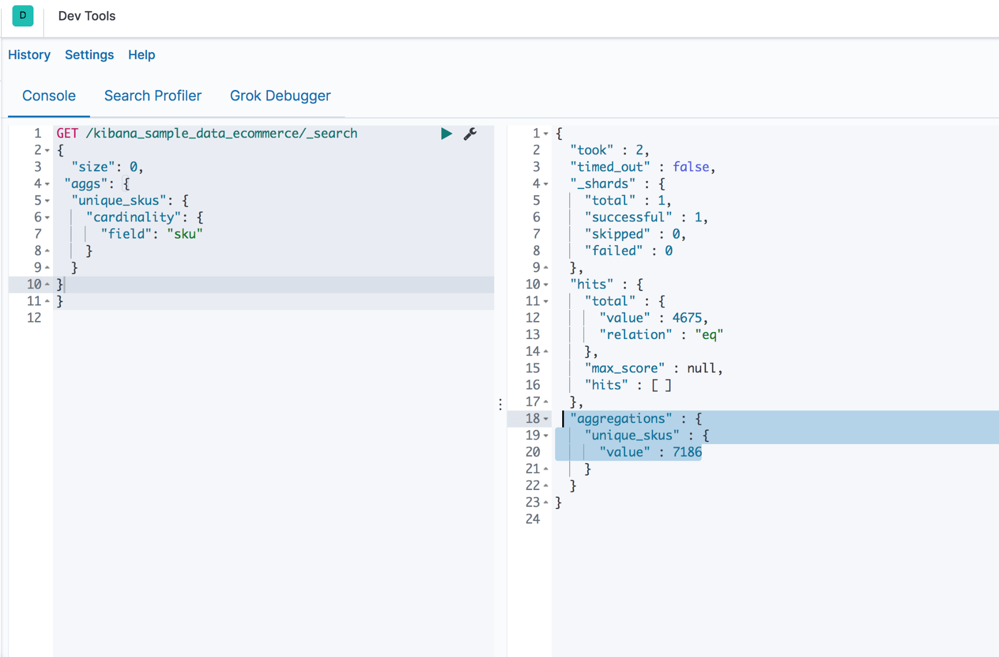
Needing to find the number of unique values for a particular field is a common requirement. The cardinality aggregation can be used to determine the number of unique elements.
Let’s see how many unique sku’s can be found in our e-commerce data.
GET /kibana_sample_data_ecommerce/_search
{
  "size": 0,
 "aggs": {
  "unique_skus": {
    "cardinality": {
      "field": "sku"
    }
  }
}
}
The cardinality aggregation response for the above code is shown in Screenshot E.
Output
You can see the same result in Kibana UI as well. We have used a Goal Chart here, which you can see in Screenshot F.

Stats Aggregation
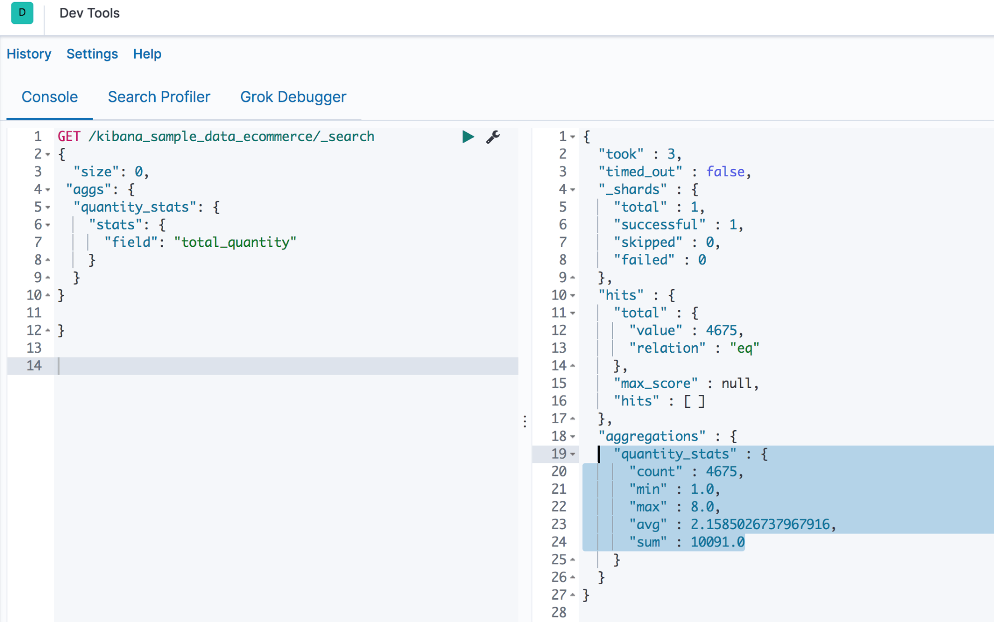
Statistics derived from your data are often needed when your aggregated document is large. The statistics aggregation allows you to get a min, max, sum, avg, and count of data in a single go. The statistics aggregation structure is similar to that of the other aggregations.
Let’s check the stats of field “total_quantity” in our data.
GET /kibana_sample_data_ecommerce/_search
{
  "size": 0,
 "aggs": {
  "unique_skus": {
    "cardinality": {
      "field": "sku"
    }
  }
}
}
Output
Screenshot G shows the stats for the quantity field—min, max, avg, sum, and count values.
You can get the same statistical results from Kibana UI, as shown in Screenshot H.

Filter Aggregation
As its name suggests, the filter aggregation helps you filter documents into a single bucket. Within that bucket, you can calculate metrics.
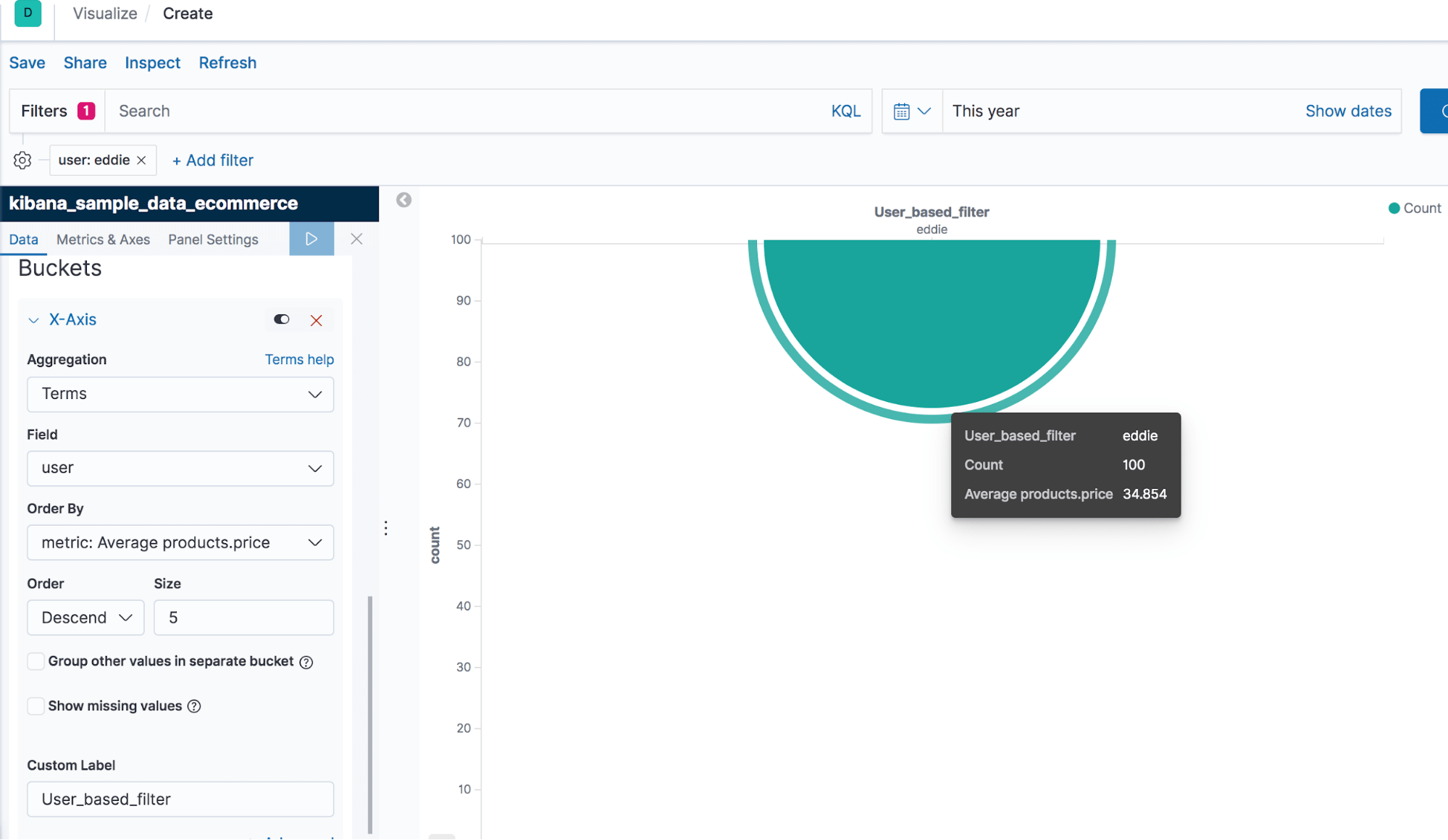
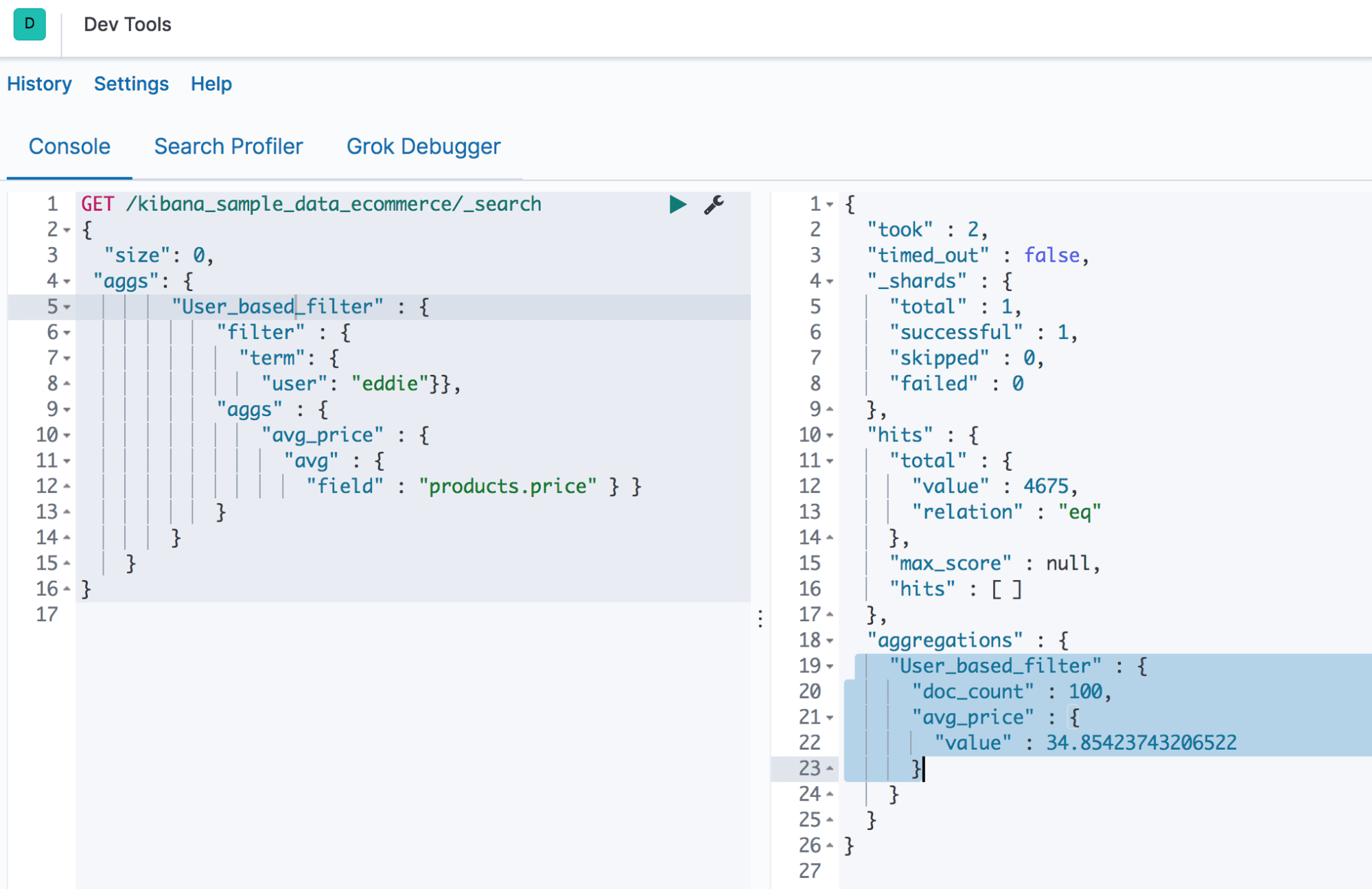
In the example below, we are filtering the documents based on the username “eddie” and calculating the average price of the products he purchased. See Screenshot I for the final output.
GET /kibana_sample_data_ecommerce/_search
{ "size": 0,
 "aggs": {
        "User_based_filter" : {
            "filter" : {
              "term": {
                "user": "eddie"}},
            "aggs" : {
                "avg_price" : {
                  "avg" : {
                    "field" : "products.price" } }
            }}}}
Output

Kibana UI Output
We have used the Line Chart to visualize the filter aggregation. To implement the filter aggregation, we first had to establish the filter “eddie” (see the top left corner in Screenshot J).
Output

Kibana UI Output
Kibana UI Output
We have used the Line Chart to visualize the filter aggregation. To implement the filter aggregation, we first had to establish the filter “eddie” (see the top left corner in Screenshot J).

Terms Aggregation
The terms aggregation generates buckets by field values. Once you select a field, it will generate buckets for each of the values and place all of the records separately.
In our example, we have run the terms aggregation on the field “user” which holds the name of users. In return, we have buckets for each user, each with their document counts. See Screenshots K and L.
GET /kibana_sample_data_ecommerce/_search
{
  "size": 0,
 "aggs": {
        "Terms_Aggregation" : {
              "terms": {
                "field": "user"}}
            }
        }
Output

Kibana UI Output

Nested Aggregation
This is the one of the most important types of bucket aggregations. A nested aggregation allows you to aggregate a field with nested documents—a field that has multiple sub-fields.
The field type must be “‘nested’” in the index mapping if you are intending to apply a nested aggregation to it.
The sample ecommerce data which we have used up until this point hasn’t had a field with the type “nested.” We have created a new index with the field “Employee” which has its field type as “nested.”
Run the code below in DevTools to create a new index “nested_aggregation” and set the mapping as “nested” for the field “Employee.”
PUT nested_aggregation
{
  "mappings": {
    "properties": {
      "Employee": {
        "type": "nested",
      "properties" : {
       "first" : { "type" : "text" },
       "last" : { "type" : "text" },
      "salary" : { "type" : "double" }
    }}}
}}
Execute the code below in DevTools to insert some sample data into the index you have just created.
PUT nested_aggregation/_doc/1
{
  "group" : "Logz",
  "Employee" : [
    {
      "first" : "Ana",
      "last" :  "Roy",
      "salary" : "70000"
    },
    {
      "first" : "Jospeh",
      "last" :  "Lein",
      "salary" : "64000"
    },
     {
      "first" : "Chris",
      "last" :  "Gayle",
      "salary" : "82000"
    },
    {
      "first" : "Brendon",
      "last" :  "Maculum",
      "salary" : "58000"
    },
    {
      "first" : "Vinod",
      "last" :  "Kambli",
      "salary" : "63000"
    },
     {
      "first" : "DJ",
      "last" :  "Bravo",
      "salary" : "71000"
    },
    {
      "first" : "Jaques",
      "last" :  "Kallis",
      "salary" : "75000"
    }]}
Now the sample data is in our index “nested_aggregation.” Execute the following code to see how a nested aggregation works:
GET /nested_aggregation/_search
{
  "aggs": {
    "Nested_Aggregation" : {
              "nested": {
                "path": "Employee"
              },
    "aggs": {
      "Min_Salary": {
        "min": {
          "field": "Employee.salary"
        }
      }
    }
}}}
Output

As you can see in Screenshot M, we have successfully called the sub-fields/nested fields of the main field “Employee.”
Note: There is no option to visualize the result of nested aggregation on Kibana UI.
Summary
This article has detailed a number of techniques for taking advantage of aggregations. There are other versions of aggregations which you might find useful as well. Some of these include:
- Date histogram aggregation—used with date values.
- Scripted aggregation—used with scripts.
- Top hits aggregation—used with top matching documents.
- Range aggregation—used with a set of range values.
As a next step, consider immersing yourself in these aggregations to find out how they might help you meet your needs. You can also visit Elastic’s official page on Aggregations.
You Might Also Like

What’s New at Logz.io – January 2026